Back to: Introduction to R
Many of the previous characteristics are the same for both axes and legends. Legends can:
Display multiple aesthetics from multiple layers
Appear in many different locations.
Can be sized and ordered differently.
You can also choose what is placed in a legend. We use the show.legend command to do this.
ggplot(df, aes(y, y)) +
geom_point(size = 4, colour = "grey20") +
geom_point(aes(colour = z), size = 2)
ggplot(df, aes(y, y)) +
geom_point(size = 4, colour = "grey20",
show.legend = TRUE) +
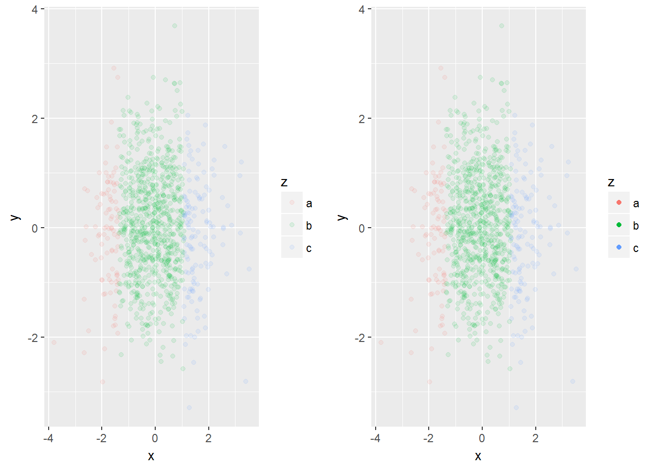
geom_point(aes(colour = z), size = 2)Sometimes we wish to have the legends display different things. For example if we use transparent colors in the plot we may want solid colors in the legend. The alpha command will make the colors more transparent. However we can override the legend colors and set the alpha differently:
norm <- data.frame(x = rnorm(1000), y = rnorm(1000))
norm$z <- cut(norm$x, 3, labels = c("a", "b", "c"))
ggplot(norm, aes(x, y)) +
    geom_point(aes(colour = z), alpha = 0.1)
ggplot(norm, aes(x, y)) +
    geom_point(aes(colour = z), alpha = 0.1) +
    guides(colour = guide_legend(override.aes = list(alpha = 1)))
The graph below shows the graph on the left where we let R create the legend. Then the graph on the right shows our changes and overriding on the colors.
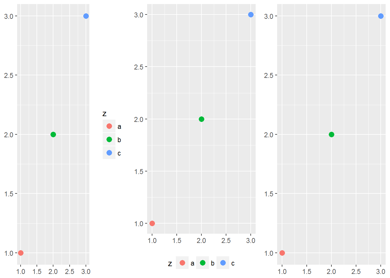
Legend Layouts
We can choose the specific layout of the legend. For example we can place it at the “top”, “bottom”, “right” , “left” or not even have a legend at all.
df <- data.frame(x = 1:3, y = 1:3, z = c("a", "b", "c"))
base <- ggplot(df, aes(x, y)) +
    geom_point(aes(colour = z), size = 3) +
    xlab(NULL) +
    ylab(NULL)
base + theme(legend.position = "right") # the default
base + theme(legend.position = "bottom")
base + theme(legend.position = "none")