Back to: Introduction to R
If we consider just looking at continuous variables we become interested in understanding the distribution that this data takes on. We will explore continuous data using:
geom_histogram() shows us the distribution of one variable.
geom_freqplot uses lines rather than boxes to show the distribution.
Histograms
Another very common graphic that most people have seen and used is the histogram. This is common among continuous data where the data is split up into bins and the frequency of those bins is displayed. They are not to be confused with bar charts though! There are no gaps in a histogram. We can add a histogram layer simply by using the geom_histogram(), if we would like to specify the width of bins we can do that by using binwidth=__:
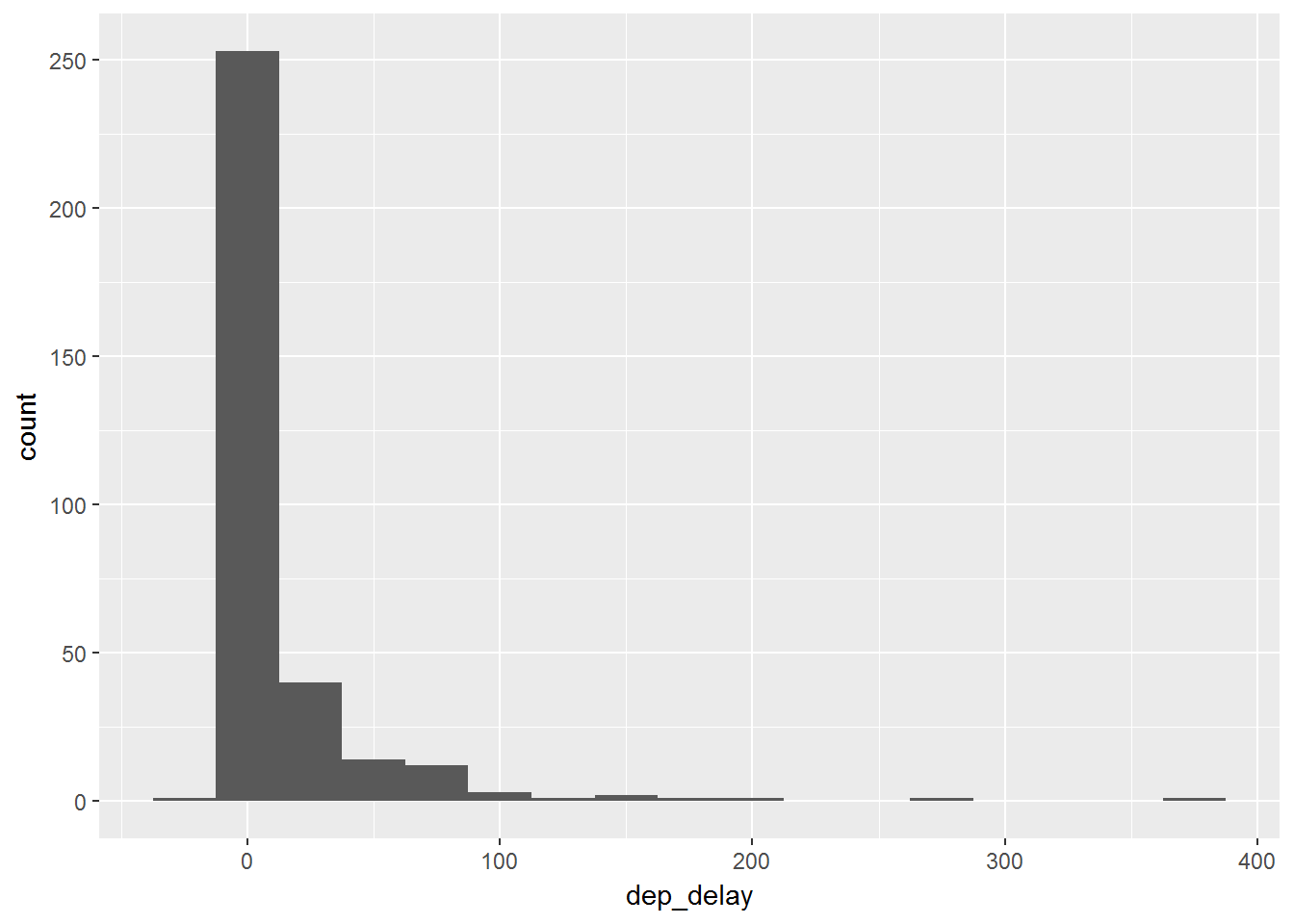
ggplot(data, aes(dep_delay)) +
geom_histogram(binwidth=25)
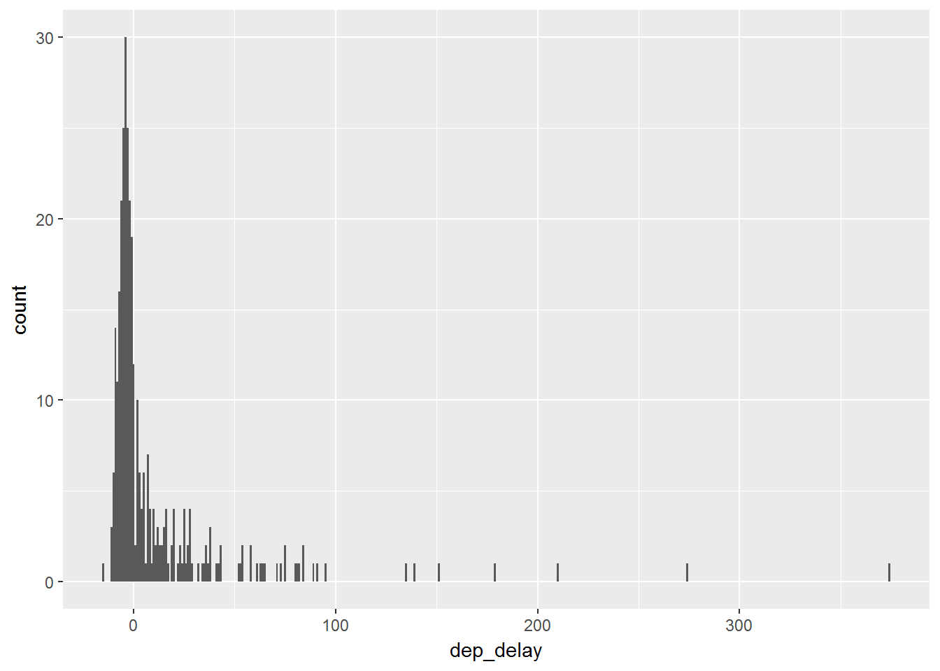
ggplot(data, aes( dep_delay)) +
geom_histogram(binwidth=1)We can see that if we use he first part of the code that we have a bin width of 25:
If we wanted to allow for more preciseness then we could use the bin width of 1:
Frequency Plots
Frequency plots are very similar to histograms. Instead of just having bars to display the frequency in a bin, the frequency plot would place a point at the height of the bar and then connect them with lines. We can simply add this with the geom_freqpoly() layer. We again can use the binwidth=__ command:
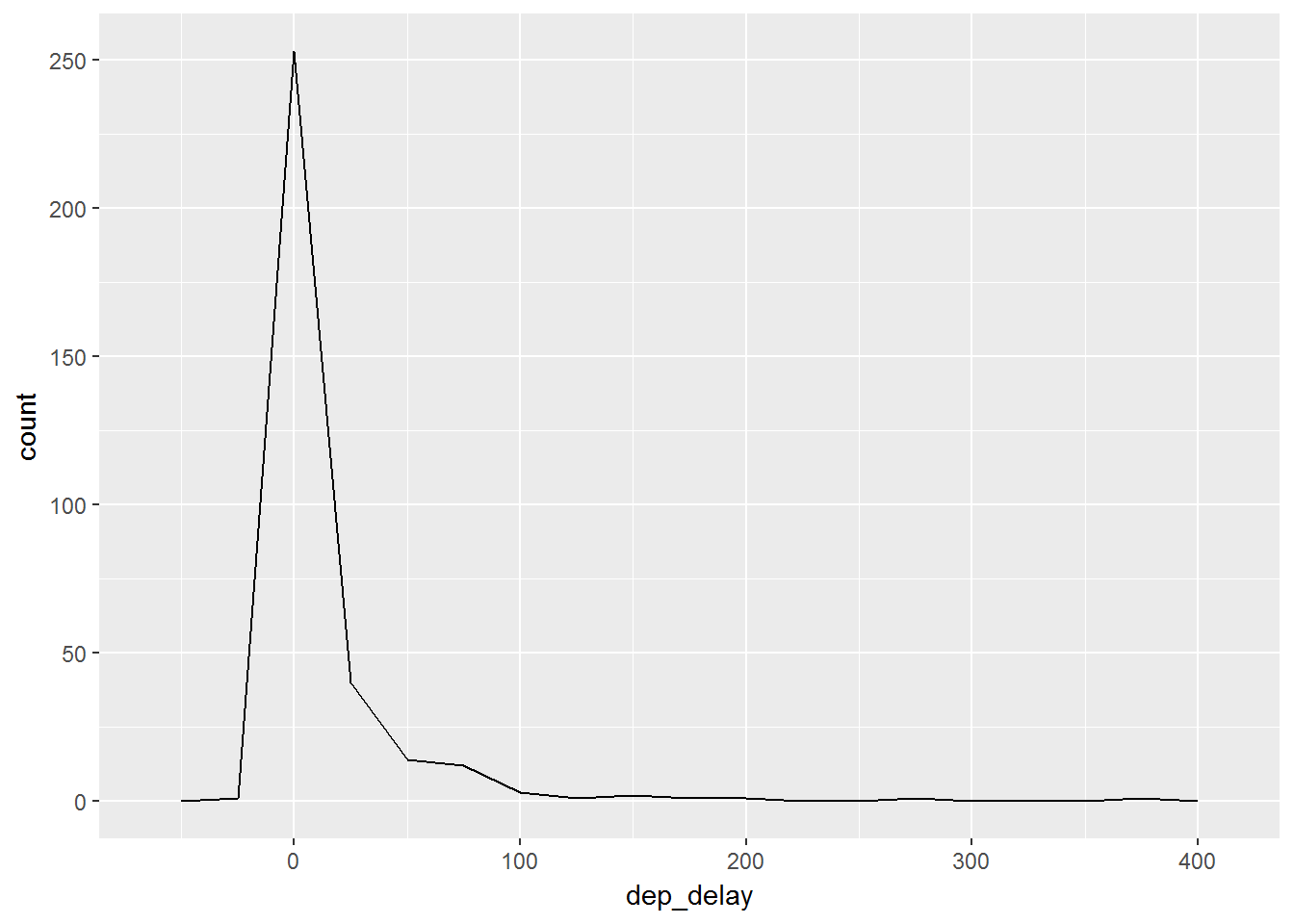
ggplot(data, aes(dep_delay)) +
geom_freqpoly(binwidth=25)
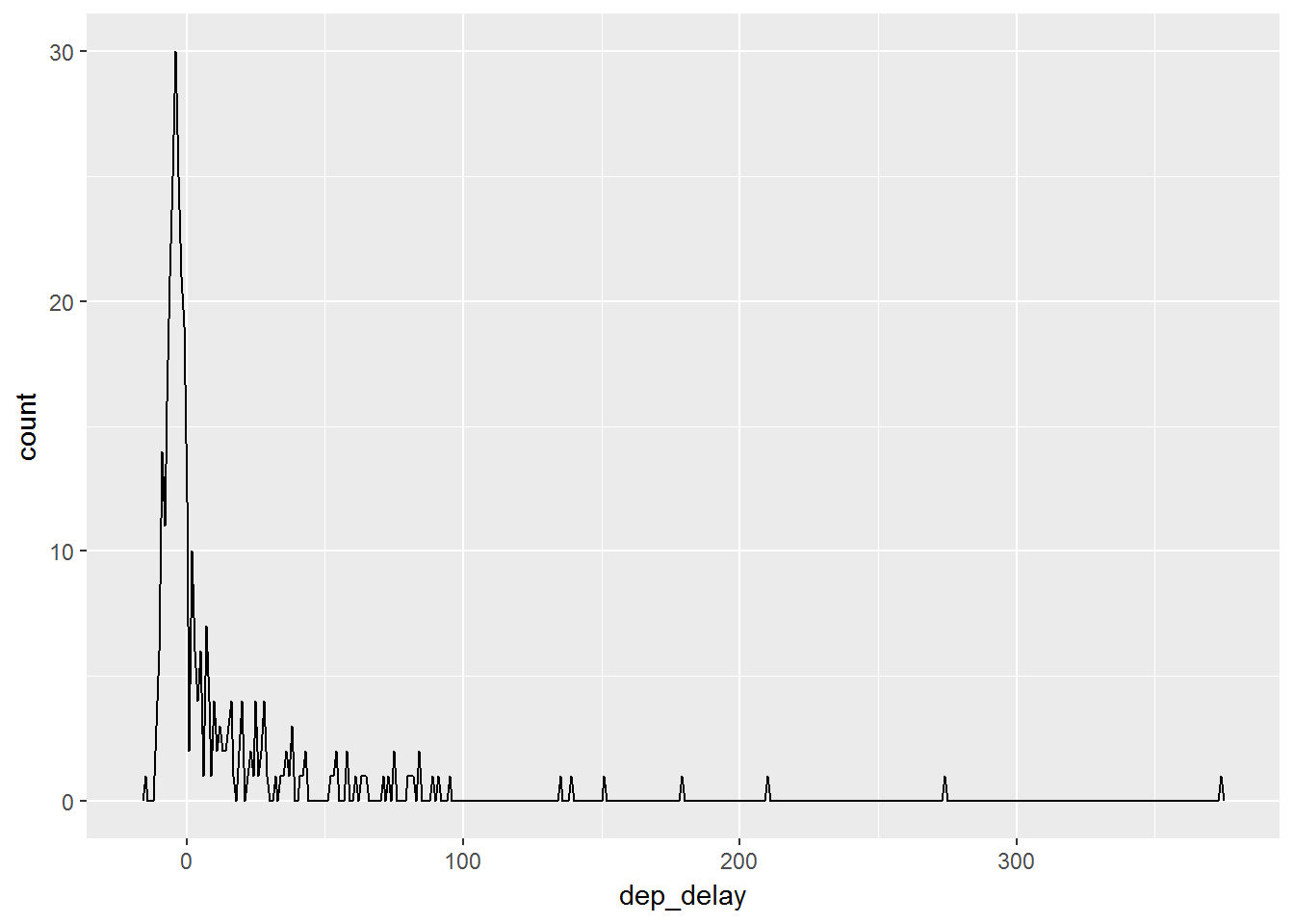
ggplot(data, aes( dep_delay)) +
geom_freqpoly(binwidth=1)With the bin width of 25 we can see the frequency plot for this:
We can also use a more precise bin width.
Adding Aesthetics
Just like in the earlier part of this unit we saw that it was possible to add a great deal of aesthetics to plots. We will now view how these changes work on these geom_ functions:
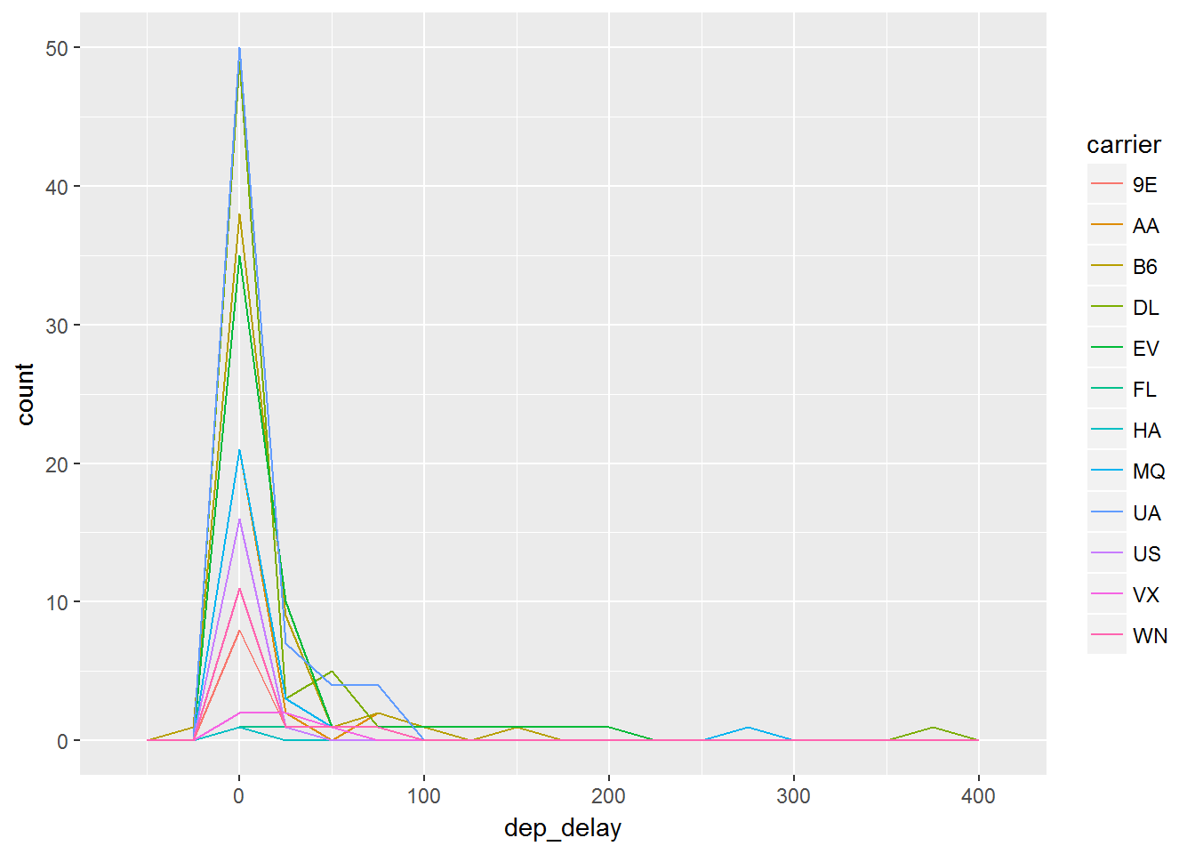
ggplot(data, aes(dep_delay, color=carrier)) +
        geom_freqpoly(binwidth=25)
If we add grouping color by carrier we can see the plot below. Notice that we now have multiple frequency plots without having to use faceting.
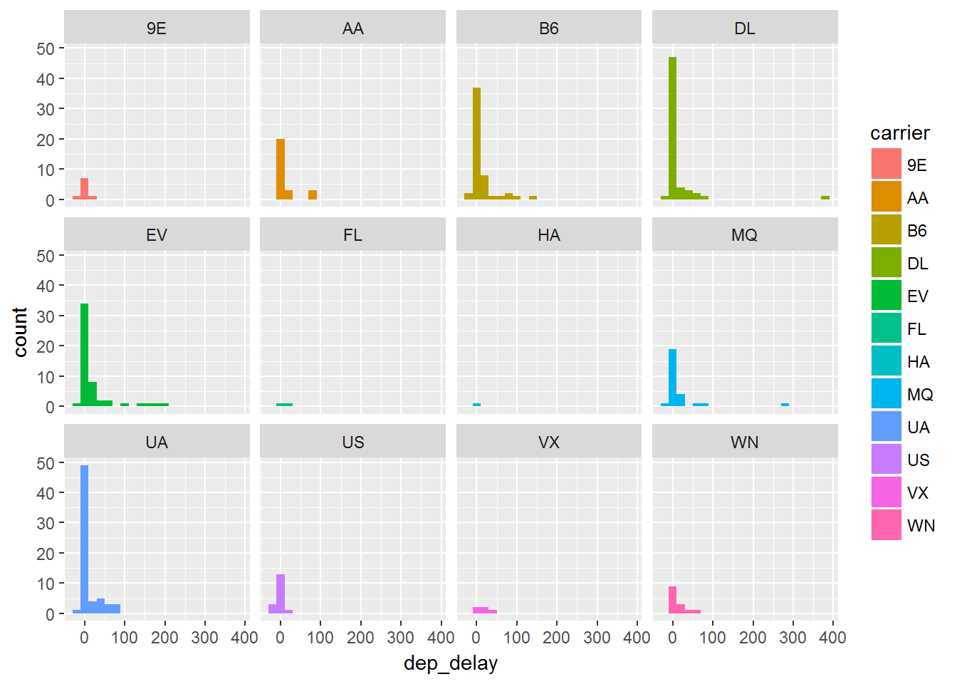
Instead of just coloring the lines, we can use the fill=__ function in order to fill a color by carrier in this case. Then we create histograms and finally in order to separate the plots out so we can see things better we use facetting:
ggplot(data, aes( dep_delay, fill = carrier)) +
        geom_histogram(binwidth=20) +
        facet_wrap(~carrier)